Author: Stuart Laurence, Department of Aerospace Engineering, University of Maryland, College Park

1 Introduction

When a hypersonic vehicle travels through the atmosphere, a boundary layer develops in the air close to the vehicle surface. Initially (close to the nose of the vehicle) this boundary layer is laminar, but typically will transition to turbulence at some point downstream. A turbulent boundary layer produces significantly larger heat flux and frictional drag at the vehicle surface than a laminar one, so to be able to accurately predict vehicle performance, knowledge of the laminar-to-turbulent transition process is important. There are a variety of boundary-layer instabilities whose growth and breakdown can lead to transition; for slender planar or axisymmetric bodies and small incidences, a key instability mechanism is the second or Mack mode, which can be thought of physically as acoustic waves that become trapped within the boundary layer. Second-mode waves typically exhibit very high frequencies – around 100 kHz or even higher – which makes their measurement very difficult with conventional techniques. Here I describe measurements of the second-mode instability using a schlieren system incorporating a CAVILUX pulsed-diode laser.

2 Experimental configuration

Experiments were performed at two hypersonic wind tunnels: the High Enthalpy Shock Tunnel Goettingen (HEG) of the German Aerospace Center (DLR), and Hypervelocity Tunnel 9 of the Arnold Engineering Development Center (AEDC) at White Oak, Maryland. HEG is capable of reproducing the extremely high flow velocities typical of atmospheric reentry (up to 7 km/s), though for very short test periods (~1 ms). In the present experiments, the flow velocity and density were 4.4 km/s and 0.0175 kg/m3. Tunnel 9, on the other hand, can produce high Mach numbers with longer test periods (around 1 s), but with lower flow velocities. In the present Tunnel 9 experiments, a variety of flow conditions were used, all having a Mach number of approximately 14 and a flow speed of 2 km/s.

In both cases the test article was a slender, 7° half-angle cone. The flow within the boundary layer over the cone was visualized using a conventional Z-fold schlieren arrangement, as shown in figure 1.

Figure 1: Z-fold schlieren visualization set-up used in the experiments described here.

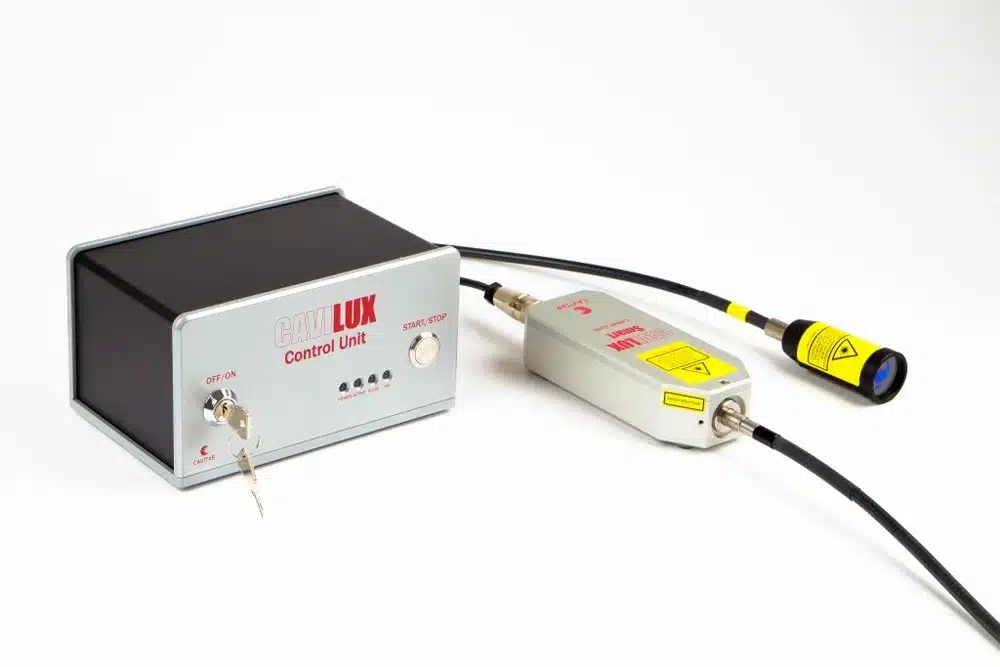
Schlieren is a technique used to visualize flow features in compressible flows: a density gradient at some location in the imaging plane within the test section (in a direction normal to the knife edge placed in front of the camera) will result in a change in intensity at the corresponding location on the image taken by the imaging device (in this case a high-speed camera). In the HEG experiments the light source was a CAVILUX Smart pulsed-diode laser and the camera was a Vision Research Phantom v1210, recording at 200 kHz. The laser was run in ultra-high-speed mode, with a repeated 4-pulse pattern as shown in figure 2.

Figure 2: Laser pulse pattern used in the HEG experiments: Δt12 is 2 μs and Δt34 is 3 μs.

This pattern was necessary because the characteristic frequency of the second-mode disturbance in this case (~600 kHz) was significantly higher than the recording frequency, so closely spaced pulse pairs were used to unambiguously resolve the wave motion (further details to be provided shortly). In the Tunnel 9 experiments, a CAVILUX HF laser providing, uniformly spaced pulses at approximately 70 kHz, was used together with a Phantom v2512 camera. The laser pulse width in the two experiments varied between 20 ns and 50 ns; such short pulse widths were necessary to freeze the high-speed flow structures in images.

3 Results

The HEG experiments were particularly challenging because of the high flow velocity (meaning high second-mode frequencies) and low density (meaning weak intensity variations in the schlieren images). An example of a visualized second-mode wave packet, visible from its oblique “rope-like” structures close to the surface, is shown as it propagates within a sequence of schlieren images in figure 3. The propagation speed of the wave packet is constant – the apparently uneven motion is a result of the laser pulse pattern. By performing two-dimensional image correlations, it is possible to recover the propagation speed – in this case it is 3.8 km/s. The unequal spacing between the two pulse pairs in figure 2 avoids problems with aliasing in these correlations. By then taking the Fourier transform of rows of pixels parallel to the cone surface, wavenumber spectra can be constructed; these can subsequently be converted into frequency spectra using the propagation speed calculated earlier.

Figure 3: Sequence of reference-subtracted schlieren images showing the propagation of a second-mode wave packet (flow is left to right)

Plots of the averaged power spectral density (PSD) at three locations downstream are shown in the left plot of figure 4. Here we see a strong peak at approximately 600 kHz – this corresponds to the second-mode frequency at these conditions. The peak grows rapidly as we move downstream, showing strong amplification of the second mode. A more detailed picture of this growth is shown in the right plot of figure 4, which is a contour plot of the PSD versus distance downstream. Further details of these measurements can be found in Laurence et al. (2016).

Figure 4: (Left) Plots of the schlieren power spectral density (PSD) near the surface at three locations downstream (s is the distance along the cone from the nose); (right) contour plot of the PSD versus distance downstream.

An example of a propagating second-mode wave packet in one of the Tunnel 9 experiments is shown in figure 5. Again we see the characteristic “rope-like” structures, though now the disturbance energy appears to be less concentrated towards the cone surface than it was in the HEG experiments.

Figure 5: Propagation of a second-mode wave packet in a Tunnel 9 experiment

In the Tunnel 9 experiments, the schlieren system was calibrated by placing a long-focal-length lens in the imaging plane and recording images of it. This enabled a calibration curve relating image intensity to the density gradient to be established. From this calibration curve, one can then quantify the growth rate of the second-mode instability. A contour plot of the integrated growth rate, or N-factor, versus distance downstream and frequency is shown in figure 6.

Figure 6: Contour plot of N-factor versus distance downstream and frequency in Tunnel 9 experiment.

Again we see a strong second-mode contribution, but now at a much lower frequency of approximately 100 kHz. The decrease in this frequency moving downstream is associated with the thickening of the mean boundary layer. Such quantitative measurements are very important as they provide data against which numerical simulations and stability analysis computations can be compared. Further details of the Tunnel 9 experiments can be found in Kennedy et al. (2017).

4 Conclusions

The experiments described here demonstrate that it is possible to use high-speed schlieren techniques to perform quantitative measurements of extremely high-frequency instability waves in hypersonic boundary layers. The capabilities of CAVILUX pulsed-diode laser light sources proved instrumental in enabling these measurements.

5 References

Kennedy, R., Laurence, S., Smith, M., and Marineau, E. (2017), ”Hypersonic Boundary-Layer Transition Features from High-Speed Schlieren Images”, 55th AIAA Aerospace Sciences Meeting, AIAA SciTech Forum, AIAA Paper 2017-1683

Laurence S., Wagner, A., and Hannemann, K. (2016), “Experimental study of second-mode instability growth and breakdown in a hypersonic boundary layer using high-speed schlieren visualization”, Journal of Fluid Mechanics, vol. 797, pp. 471-503

About the author

Stuart Laurence (Ph.D) completed his graduate studies at the Graduate Aeronautical Laboratories, California Institute of Technology, in the area of hypersonic flows. He currently is Assistant Professor at the Department of Aerospace Engineering, University of Maryland, College Park